This page introduces the typical application of Repeated Measures ANOVA and the reporting of the findings.
A brief introduction to the study:
Several studies have examined the effects of cocaine exposure to the health of new babies. These studies reported that the average birth weight for babies with cocaine exposure was less heavy than that for babies without cocaine exposure. Suppose a researcher was interested not only in birth weight, but also in assessing whether the growth rates were slower for babies with cocaine exposure. She collected data from early born babies at birth and then once a week after birth for a total of four measures. After excluding outliers (extremely short and light babies), she had a total of 95 later born babies whose moms used cocaine during gestation and 97 later born babies whose moms reported no drug use during pregnancy. The dependent variable was babies' weight in grams. Babies with missing values on any of the repeated measures were list-wise deleted from the dataset.
Results:
Repeated Measures ANOVA was used to test the hypothesis whether babies with cocaine exposure were less heavy and had slower growth rates than babies without cocaine exposure. The dependent variable in the study was weight in grams repeatedly measured for four times. The between-subject independent variable was Group indicating babies with and without cocaine exposure. The within-subject independent variable was Week indicating time of data collection at 0, 1, 2, and 3 weeks.
Outliers were examined using the criterion that any z score great than 3 or less than -3 on the dependent variable was a univariate outlier. Multivariate outliers were examined using the Mahalanobis Distance Test with p value < 0.01. No outlier was found in the dataset (probably because the dataset had been previously screened for outliers). Normality assumption was examined using the skewness indices on repeated measures within each group. All skewness indices were found in proper ranges from -1 to +1, indicating an approximate normality. However, the Mauchly Test of Sphericity Assumption was significant (p < 0.01) showing violation of this assumption. An adjusted test (The Huynh-Feldt Test) was used to report more accurate findings. Carry-Over effect was not an issue in this study because a previous measure of weight was not likely to influence the follow-up measures.
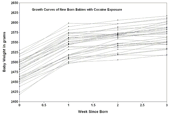
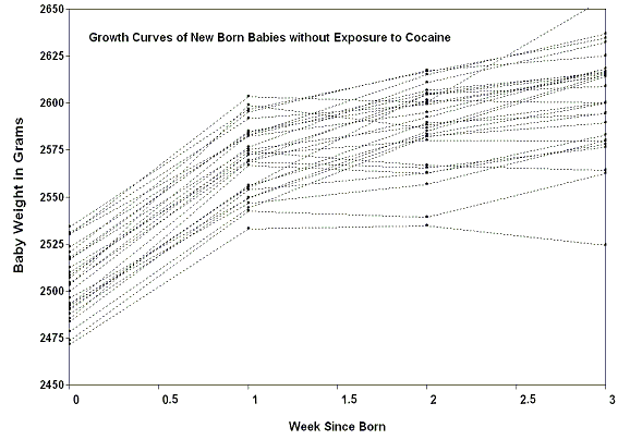
Exploratory data analysis was conducted using line graphs. Figure 1 shows individual growth curves in the four weeks for babies with and without cocaine exposure. It can be seen from Figure 1 that babies with cocaine exposure were less heavy at birth and had a slightly flatter curve than babies without cocaine exposure. It is also of interest to see that at the end of fourth week, the babies without cocaine exposure had greater variance in weight than the babies with cocaine exposure.
Figure 1
Developmental Curves of New Born Babies With ( N = 95) and Without (N = 97) Cocaine Exposure


|
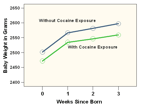
Figure 2 presents the average growth trajectories for babies with and without cocaine exposure in the first four weeks. It is clear from Figure 2 that the average weight was lighter for the babies with cocaine exposure at each repeated measure. More importantly, the difference between the average weights became wider as time went on, indicating that the growth rates for babies with cocaine exposure were slower than that for babies without cocaine exposure.
Figure 2
Line Graphs of New Babies Weight Measured Four Times after Birth for Babies With and Without Exposure to Cocaine
|
Two main effects and one interaction effect were tested using Repeated Measures ANOVA. The main effect of Group concerned the hypothesis that the two groups were different in weight regardless of measurement times. The main effect of Week evaluated the hypothesis that baby weight was different at different times of measurement regardless of group effect. The interaction term examined whether babies with and without cocaine exposure were different in their growth in the first four weeks. It was this interaction term that was most interesting to the researcher.
Results from Repeated ANOVA were presented in Table 1. Since the Sphericity Assumption was violated, results from the Huynh-Feldt Test was reported for adjusting the p-values for increased accuracy. It can be seen from Table 1 that the two main effects and the interaction term were all significant at p < 0.001 level. A significant Group effect showed that the average weight was significantly greater for babies without cocaine exposure in the first four weeks (also see Figure 2). A significant main effect of Week indicated that the weight was significantly different at different measurement combining two groups together. Since this result was not of direct interest to the researcher (because it combines two groups together), no post hoc test was further conducted). A significant interaction term revealed that babies with and without cocaine exposure were significantly different in their growth rates during the four weeks. It can be seen from Figure 2 that the curve was slightly flatter for babies with cocaine exposure, indicating a slower growth rate.
Table 1
The Summary Table of Repeated Measures ANOVA for the Birth Weight Data
| Source | Degrees of Freedom | F | p - value |
| Week | 2.64, 501.7 | 3904.4 | < 0.001 |
| Group | 1, 190 | 88.1 | < 0.001 |
| Week x Group | 2.64, 501.7 | 6.7 | < 0.001 |
Means and standard deviations for the weight measured at different times are presented in Table 2. The Independent Samples t test was performed to compare mean difference for each repeated measure for the two groups. Table 2 shows that babies without cocaine exposure were heavier than the babies with cocaine exposure at each measurement time. In summary, the Repeated Measures ANOVA revealed that babies with cocaine exposure were less heavy and grew slower than babies without cocaine exposure.
Table 2
Means and Standard Deviations of Babies Weight (in grams) Measured Repeatedly for Four Weeks after Born with and without Cocaine Exposures
| Week 0 | Week 1 | Week 2 | Week 3 | |
| Without Exposure | 2501.8 (19.8) | 2567.2 (20.3) | 2581.4 (23.3) | 2597.4 (26.2) |
| Without Exposure | 2471.9 (28.9)** | 2536.8 (28.7)** | 2546.4 (29.4)** | 2559.8 (29.9)** |
To download the source data, please click here.