This page introduces the typical application of Logistic Regression and the reporting of the findings.
A brief introduction to the study:
Many studies have presented models to predict whether a married woman is in the paid labor force. For example, Long (1997) used Logistic Regression to examine whether the number of children with age 5 or younger, the number of children ages 6 to 18, the woman's age, the wife or the husband's education, estimated wage rate and family income (excluding wife's wage) were associated with the woman's current employment status. Data were extracted from the 1976 Panel Study of Income Dynamics. The sample consisted of 753 white, married women between age 30 and 60. The dependent variable Employment was coded 1 or 0 indicating Yes or No for the woman's employment status. Education was coded in a dummy variable indicating whether the husband or the wife spent at least one year in college, rather than the more traditional measures of how many years in school.
The researcher was interested in identifying significant predictors of a woman being in the paid labor force. It was also of interest to examine moderators of joining in the labor force. For example, if a woman's age was significantly related to the probability of being in the labor force, was this relationship different for women with different educational levels? In this case, Education was evaluated as the moderator between the probability of being in the labor force and a woman's age.
Results:
Logistic regression was used to build a model for predicting whether married women were currently employed full-time in the paid labor force. The dependent variable was a dichotomous variable with 1 indicating full-time employment and 0 indicating otherwise. Independent variables included both continuous and categorical variables. The continuous independent variables were the number of children at home with age 5 or younger, the number of children with ages from 6 to 18, the wife's age and total family income excluding the wife's expected income. Categorical independent variables were whether the wife or the husband attended college. The sample contains 753 married women. SPSS version 13 was used to conduct the logistic regression analyses and to produce the figure.
Prior to conducting logistic regression, the normality assumption was examined using the skewness index for each continuous variable. Wife's estimated wage rate was found positively skewed, and therefore, a logarithmic transformation was performed to convert the variable into approximately normal.
Table 1 presents descriptive statistics of the variables in the logistic regression model. We can see from Table 1 that the dependent variable was approximately balanced with 57% reported in the labor force and 43% not employed. It should be noted that although the standard deviations of dichotomous variables are conventionally presented in a descriptive statistics table, no straightforward interpretation for a standard deviation of a categorical variable. For example, the standard deviation for Employment is 0.50 which had no direct interpretation.
Table 1
Means and Standard Deviations for the Labor Force Participation Example (N = 753)
| Mean | STD | Minimum | Maximum | |
| Employment | 0.57 | 0.50 | 0.00 | 1.00 |
| Children ages 5 or younger | 0.24 | 0.52 | 0.00 | 3.00 |
| Children ages 6 to 18 | 1.35 | 1.32 | 0.00 | 8.00 |
| Wife's age in years | 42.54 | 8.07 | 30.00 | 60.00 |
| Wife attended college | 0.28 | 0.45 | 0.00 | 1.00 |
| Husband attended college | 0.39 | 0.49 | 0.00 | 1.00 |
| Log of wife's wage rate | 1.10 | 0.59 | -2.05 | 3.22 |
| Family income | 30.13 | 11.63 | -0.03 | 96.00 |
Results from logistic regression are presented in Table 2. Table 2 shows that the number of children age 5 or younger, the wife's age, education, log of estimated wage rate and family income were significant predictors of whether a woman was currently in the paid labor force. Number of children ages 6 to 18 and husband's education were not significant predictors. Unstandardized estimates can be used for interpreting results from a logistic regression. For example, the unstandardized estimate for the number of children age 5 or younger is -1.463, indicating that an increase of each child younger than 6 is associated with a decrease of -1.463 in the logit of the probability in the labor force, holding all other variables constant.
Since logit is a scale unfamiliar to most people, odds ratio (OR) is often used for interpretation. For example, an OR of 0.232 for younger children indicated that for each additional young child, the odds of being employed were decreased by a factor of 0.232, holding all other variables constant. Or equivalently, for each additional young child, the odds of working fulltime would decrease 77% holding all other variables constant. For OR greater than 1, it is necessary to subtract 1 from the estimated OR to make a better interpretation. For example, the estimated OR for wife's education is 2.242, indicating that the OR to be employed for a wife attended college is 1.242 times greater than a wife without attended college. Upper and lower 95% confidence intervals for odds ratios are also presented in Table 2. Please note that confidence intervals are directly related to sample sizes: larger sample sizes will result in narrower range of confidence intervals.
Table 2
Results from Logistic Regression Analysis of Labor Force Participation
|
Variable |
B |
S.E. |
p |
Odds Ratio |
Lower 95% CI |
Upper 95% CI |
|
Intercept |
3.182 |
0.644 |
0.000 |
24.098 |
|
|
|
Children ages 5 or younger |
-1.463 |
0.197 |
0.000 |
0.232 |
0.157 |
0.341 |
|
Children ages 6 to 18 |
-0.065 |
0.068 |
0.342 |
0.937 |
0.820 |
1.071 |
|
Wife's age in years |
0.063 |
0.013 |
0.000 |
0.939 |
0.916 |
0.963 |
|
Wife attended college |
0.807 |
0.230 |
0.000 |
2.242 |
1.428 |
3.518 |
|
Husband attended college |
0.112 |
0.206 |
0.588 |
1.118 |
0.747 |
1.675 |
|
Log of wife's wage rate |
0.605 |
0.151 |
0.000 |
1.831 |
1.362 |
2.460 |
|
Family income |
-0.034 |
0.008 |
0.000 |
0.966 |
0.961 |
0.982 |
The accuracy of prediction performed by a logistic regression can be evaluated using a classification table, presented in Table 3. Table 3 shows that about 80% of the women who were in the labor force were correctly predicted by the logistic regression, but only 55.4% of the women who were not in the labor force were correctly predicted. The overall percentage of prediction accuracy is 69.3%.
Table 3
Classification Table for Logistic Regression on Labor Force participation
| ĪĪ | Predicted | ĪĪ | |||
| ĪĪ | Yes | No | Total | % correct | |
| Observed in Labor Force: | Yes | 342 | 86 | 428 | 79.9 |
| No | 145 | 180 | 325 | 55.4 | |
| ĪĪ | Total | 487 | 266 | 753 | 69.3 |
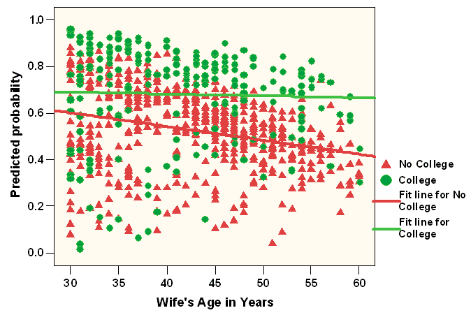
To examine whether wife's education was moderating the effect between women's age and the probability of current employment, a multiple linear regression was conducted using the predicted probability as the dependent variable, and wife's age, Education and the product term were included as the independent variables. The results from the multiple regression confirmed that wife's education is a significant moderator with p = 0.004. Figure 1 presents the scatter plot of predicted probability and Age separately by women's education status. It is clear from Figure 1 that for women who had attended college, age is not related to the probability of employment. For women who had not attended college, however, the probability of being employed decreased with increasing age.
Figure 1
Probability of Labor Force Participation by Age and Wife's Education

|
To download the source data, please click here.